ODE Solver

Description

This project is a simple ODE solver using different numerical methods, like Forward Euler, Heun's Method, and Runge-Kutta 4. Furthermore, it is possible to compare multiple methods in terms of accuracy and speed.

Goals

The goal of this project is to implement different numerical methods for solving ODEs and due to that to get a better understanding of the methods and their advantages and disadvantages.

Technologies Used

Python 3.11
Numpy (for the implementation of the methods)
Matplotlib (for the visualization of the results)
Scipy (for the comparison of the methods)
argparse (for the command line interface)

Features

Implemented Methods

Explict Methods
- Forward Euler
- Heun's Method
- Two-Step Adams-Bashforth
Explicit Runge-Kutta Methods
- Midpoint Method
- Runge-Kutta 3
- Runge-Kutta 4
- Third-Order Strong Stability Preserving Runge-Kutta
Adaptive Runge-Kutta Methods
- Adaptive Heun-Euler
- Adaptive Runge-Kutta 4/5
- Adaptive Fehlberg 1(2)
- Adaptive Dormand-Prince

Installation

To install the project, you need to have Python 3.11 installed. Then you can clone the repository and install the requirements with the following commands:

git clone https://github.com/henribe01/ODE_Solver.git
cd ODE_Solver
pip install -r requirements.txt

Usage

usage: ODE Solver [-h] -i INITIAL_CONDITIONS [INITIAL_CONDITIONS ...] [-t T_END]
                  [-m {AdaptiveRK45,AdaptiveHeunEuler,ForwardEuler,Heun,TwoStepAdamBashforth,RK4} [{AdaptiveRK45,AdaptiveHeunEuler,ForwardEuler,Heun,TwoStepAdamBashforth,RK4} ...]] [-s STEP_SIZE] [-a] [-e] [-c] [-o OUTPUT] [-sc]
                  {simple_pendulum}

Solve ODEs using different methods andcompare them

positional arguments:
  {simple_pendulum}     ODE to solve. Must be a file in the ODEs folder.The file must contain a function with the same name. The function must take the form f(x, x', ..., x^{(n-1)}, t) and return the value of x^{(n)}

options:
  -h, --help            show this help message and exit
  -i INITIAL_CONDITIONS [INITIAL_CONDITIONS ...], --initial_conditions INITIAL_CONDITIONS [INITIAL_CONDITIONS ...]
                        Initial conditions for the ODE. Must be the same length as the order of the ODE.
  -t T_END, --t_end T_END
                        Time to solve up to.
  -m {AdaptiveRK45,AdaptiveHeunEuler,ForwardEuler,Heun,TwoStepAdamBashforth,RK4} [{AdaptiveRK45,AdaptiveHeunEuler,ForwardEuler,Heun,TwoStepAdamBashforth,RK4} ...], --methods {AdaptiveRK45,AdaptiveHeunEuler,ForwardEuler,Heun,TwoStepAdamBashforth
,RK4} [{AdaptiveRK45,AdaptiveHeunEuler,ForwardEuler,Heun,TwoStepAdamBashforth,RK4} ...]
                        Methods to use for solving the ODE.
  -s STEP_SIZE, --step_size STEP_SIZE
                        Step size to use for solving the ODE.
  -a, --all             Plot all methods in one plot.
  -e, --error           Plot error vs step size.
  -c, --cpu_time        Measure CPU time vs step size.
  -o OUTPUT, --output OUTPUT
                        Output file name. If not specified, will show plot.
  -sc, --scipy          Use scipy's odeint method to solve the ODE as well.

If you want to solve your own ODE, you need to create a file in the ODEs folder with the name of your ODE. The file must contain a function with the same name. The function must take the form \(f(x, x', ..., x^{(n-1)}, t)\) and return the value of \(x^{(n)}\). Then you can use the command line interface to solve your ODE.

Challenges and Solutions

During the implementation of the project, I encountered a few challenges. One of them was the implementation for solving higher order ODEs. I solved this by creating a function, which returns a numpy array containing the derivatives of the given ODE. For the first \(n-1\) elements, the function returns the next value in the given array. For the last element, the function returns the value of the ODE at the given point. This way, the function can be used for solving any ODE of any order.

Another challenge was the implementation of a user interface. I solved this by using the argparse module, which allows for a simple implementation of a command line interface. This way, the user can easily specify the ODE to solve, the initial conditions, the methods to use, the step size, and the time to solve up to.

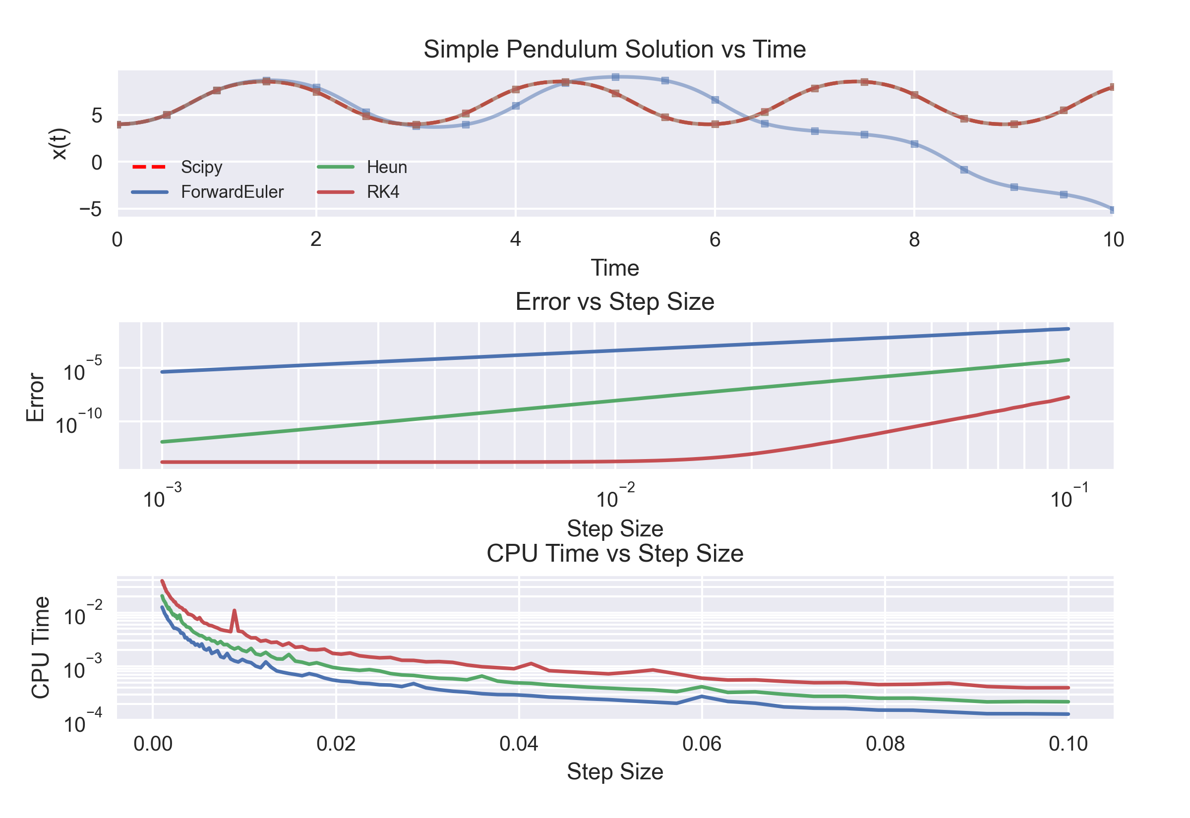
Results and Outcomes

The results of the project is, that some of the numerical methods are sometimes unstable. This means, that the error of the methods increases exponentially over time. This is the case for the Forward Euler method, which is only stable for step sizes smaller than \(0.1\).

Furthermore, the results show, that the Runge-Kutta 4 method is accurate even for larger step sizes. The downside of this method is, that it significantly slower than the other methods. This is due to the fact, that the method calculates the derivatives at multiple points between the start and the end of the step.

Ordinary Differential Equations Solver